Face Images Retrieval with Attributes Modifications
In this work I design an image retrieval system able to retrieve images similar to a query image but with some modified attributes. In our setup we employ a dataset of face images, and the attributes are annotated face characteristics, such as smiling, young, or blond. However, the proposed model and training could be used with other type of images and attributes.
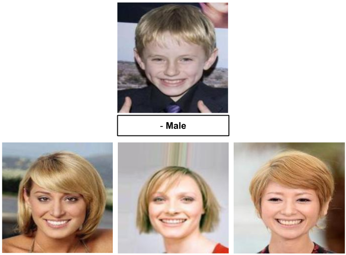
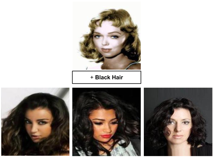
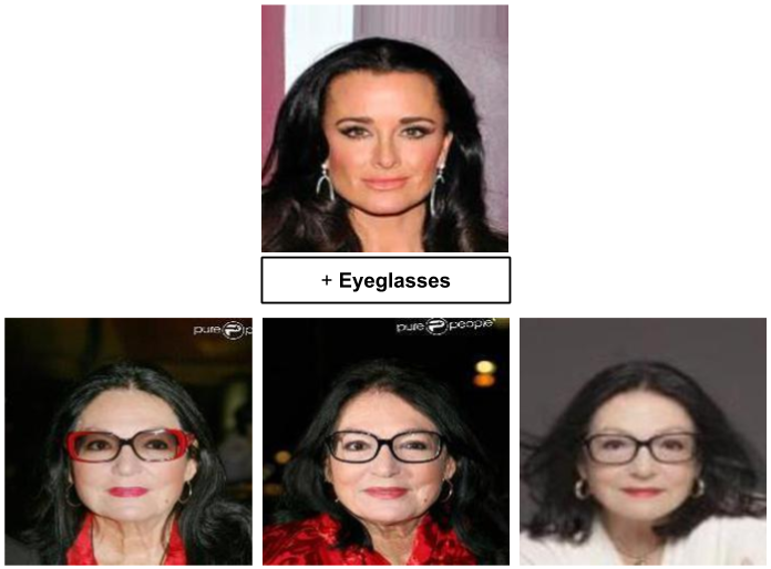
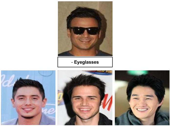
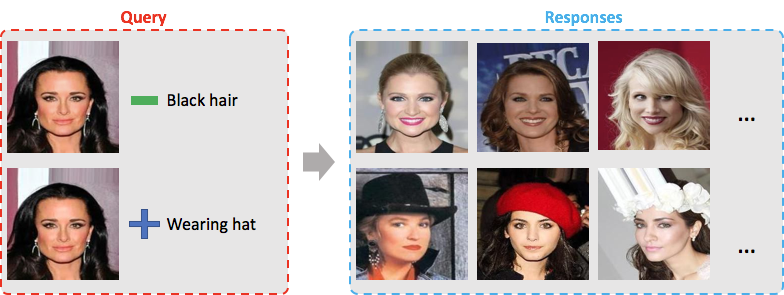
I design a model to learn embeddings of images and attributes to a joint space, test different training approaches, and evaluate if the system is able to retrieve images similar to a query image with an attribute modification, as shown in the following figure.
The code used in this work is available here.
Data
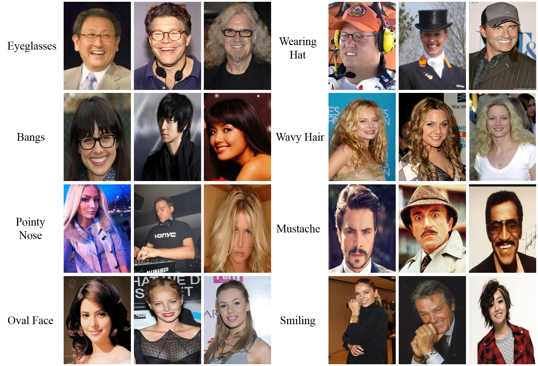
I use the Large-scale CelebFaces Attributes (CelebA) Dataset dataset which contains arround 200k celebrity face images with 40 annotated binary attributes. Standard dataset splits are employed: 162k train, 20k val and 20k test images.
-
Images: Use the already aligned and cropped images and resize them to 224x224 (to fit ResNet input size). Since they are aligned, I’ll omit data augmentation.
-
Attributes: Encoded as 40-Dimensional multi-hot vectors.
Model
The proposed model aims to learn embeddings for images and attributes vectors to a joint embedding space, where the embedding of a given image should be close to its attributes vector embedding. A pretrained ResNet-50, whose last layer has been replaced by a linear layer with 300 outputs, learns embeddings of images into out joint embedding space (which will have 300 dimensions). Attributes are processed by 2 linear layers with 300 outputs (the first one with Batch Norm and ReLu) and then embedded in the same space. Both the 300-D representations of images and attributes are L2-normalized.
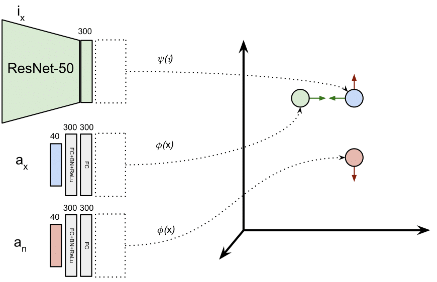
In this figure, we use a siamese setup for attribute vectors \(a_x\) and \(a_n\), so the layers processing them are actually the same (\(\phi\)).
The reason of applying L2-normalization to the embeddings is that in test time, when we operate with query image embeddings and attribute representations, we won’t need to care about the final query representation magnitude, since all the embeddings will be normalized. Normalizing embeddings reduces their discrimination capability, but given the high dimensionality of the embedding space that won’t be a problem in our setup.
Training
The model is trained with a triplet margin loss (or triplet loss, ranking loss, …). If the anchor is an image \(I_x\), the positive is its attribute vector \(a_x\), and the negative is a different attribute vector \(a_n\), the loss forces the distance between \(I_x\) and \(a_n\) in the embedding space to be larger than the distance between \(I_x\) and \(a_x\) by a margin.
For a detailed explanation of how triplet loss works, read the post “Understanding Ranking Loss, Contrastive Loss, Margin Loss, Triplet Loss, Hinge Loss and all those confusing names”.
Intuitively, the loss forces the image embedding to be closer in the embedding space to its attributes embedding than to other attribute embeddings. Therefore, the embedding of an image of a blond man, will be closer in the embedding space to the blond, man attributes than to the blond, woman attributes or to the black_hair, man attributes embedding.
I used a margin of 0.1 and an initial learning rate of 0.1, which is divided by 10 every 5 epochs.
Negatives
I used two different negatives mining strategies:
-
Random existing negatives: Random (different) attribute vector in the dataset.
-
Hard negatives: To build the negative attributes \(a_n\), change the value of 1 to 3 random attributes of the positive attributes vector \(a_x\). Empirically, I found out that this hard negatives can only be used in one third of the triplets. If they are used more, the net overfits to real attribute vectors, embedding them always closer to the image because they are real, not because their attributes match.
Retrieval
In order to use the proposed model to retrieve images similar to a query image with some modified attributes, we follow this procedure:
-
Compute the embeddings of the test images.
-
Compute the embedding of the query image.
-
Compute the embedding of the attribute vector which we want to use to modify our query image. As an example, if we want to modify the black_hair attribute and its index in our 40-dimensional attributes vector is \(0\), this vector would be [1,0,0,0,0, …].
-
Combine the query image embedding and the attribute vector embedding. If we want to change the query image to have black hair, we would sum the vectors. If our query image has black hair and we want to retrieve similar ones but with other hair colors, we would subtract the attribute vector embedding (encoding black_hair) from the query image embedding.
-
L2 normalize the resulting embedding, to ensure that, no matter the operations we have done, all the embeddings have the same magnitude.
-
Compute the distance between the modified query embedding and each test image embedding, and get the most similar images. The distances used here is the euclidean distance (torch’ PairwiseDistance) and should be the same as the one used in the loss (in this case torch’ TripletMarginLoss).
When combining query image embeddings and attribute vectors in step 4, we can do any operations we want, adding or subtracting different attributes, or even weighting image and attribute embeddings to increase their influence in the final embedding.
Evaluation
This work stayed as a fast toy experiment, so I’ve not compared its performance or methodology with related work in the field. However, I designed performance metrics to evaluate the trained models in both similarity of the retrieved images with the query image and with the desired target attributes (those are the query image attributes with the modifications). First, I generate random queries by selecting a random attribute modification for each query image. Then, I retrieve the top-10 images for those queries, and compute the following evaluation metrics:
-
Mean Correct Attributes (MCA): Mean number of results (we consider 10 per query) that have the specified attribute by the attribute modifier. This measure does not evaluate similarity with original image.
-
Mean Cosine Similarity (MCS): Mean cosine similarity of the retrieved images (10) with the query images in the embedding space. This measure does not evaluate attribute modifications.
-
Cosine Similarity P@10 (CS-P@10): A result is considered relevant if it has the attribute specified by the modifier. Then, it contributes to P@10 with its cosine similarity with the query image in the embedding space, to evaluate also the similarity with the query image. This measure evaluates both similarity with the query image and the attribute modification.
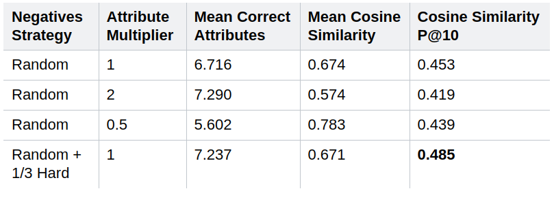
When we use an attribute multiplier of \(2\) (which means that in step 4. the weight of the attributes vector is doubled), the MCA performance increases, since we are increasing the influence of the modified attribute in the resulting embedding. Similarly, if we decrease its influence multiplying it by \(0.5\), we’ll retrieve images more similar to the query image, and so the MCS performance increases. Results also show that the hard negatives boost performance.
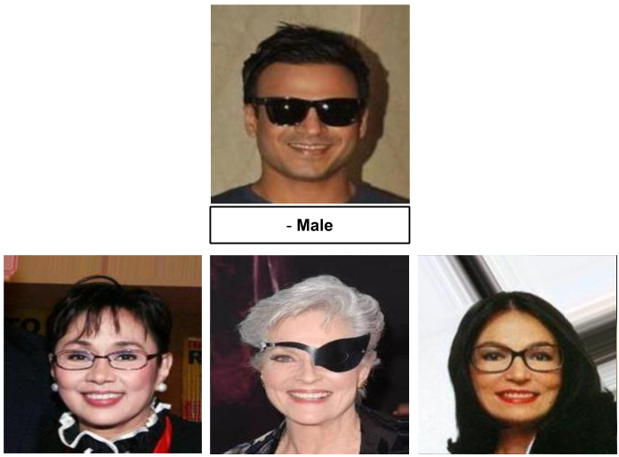
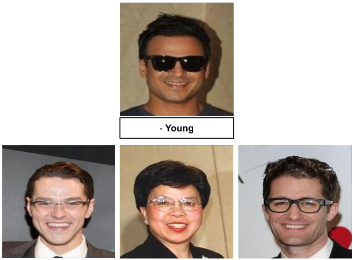
Qualitative results
Following, I show some qualitative results of the best performing model, where a query with a single attribute modification is done and the top-3 results are shown.