Understanding Categorical Cross-Entropy Loss, Binary Cross-Entropy Loss, Softmax Loss, Logistic Loss, Focal Loss and all those confusing names

People like to use cool names which are often confusing. When I started playing with CNN beyond single label classification, I got confused with the different names and formulations people write in their papers, and even with the loss layer names of the deep learning frameworks such as Caffe, Pytorch or TensorFlow. In this post I group up the different names and variations people use for Cross-Entropy Loss. I explain their main points, use cases and the implementations in different deep learning frameworks.

First, let’s introduce some concepts:

Tasks

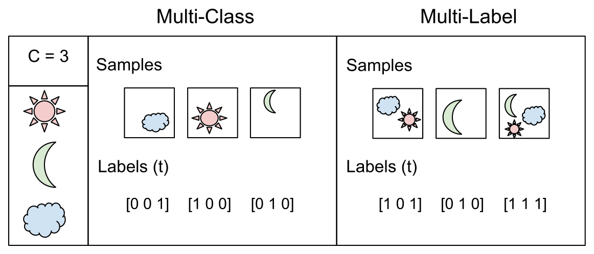
Multi-Class Classification

One-of-many classification. Each sample can belong to ONE of $C$ classes. The CNN will have $C$ output neurons that can be gathered in a vector $s$ (Scores). The target (ground truth) vector $t$ will be a one-hot vector with a positive class and $C - 1$ negative classes.
This task is treated as a single classification problem of samples in one of $C$ classes.

Multi-Label Classification

Each sample can belong to more than one class. The CNN will have as well $C$ output neurons. The target vector $t$ can have more than a positive class, so it will be a vector of 0s and 1s with $C$ dimensionality.
This task is treated as $C$ different binary $(C’ = 2, t’ = 0 \text{ or } t’ = 1)$ and independent classification problems, where each output neuron decides if a sample belongs to a class or not.

Output Activation Functions

These functions are transformations we apply to vectors coming out from CNNs ($s$) before the loss computation.

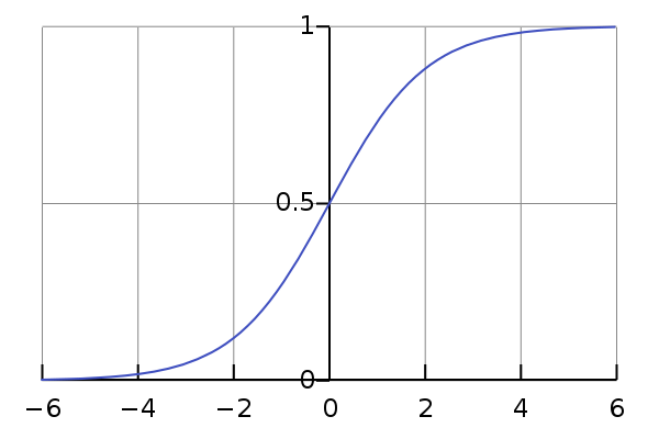
Sigmoid

It squashes a vector in the range (0, 1). It is applied independently to each element of $s$ $s_i$. It’s also called logistic function.

$f(s_{i}) = \frac{1}{1 + e^{-s_{i}}}$

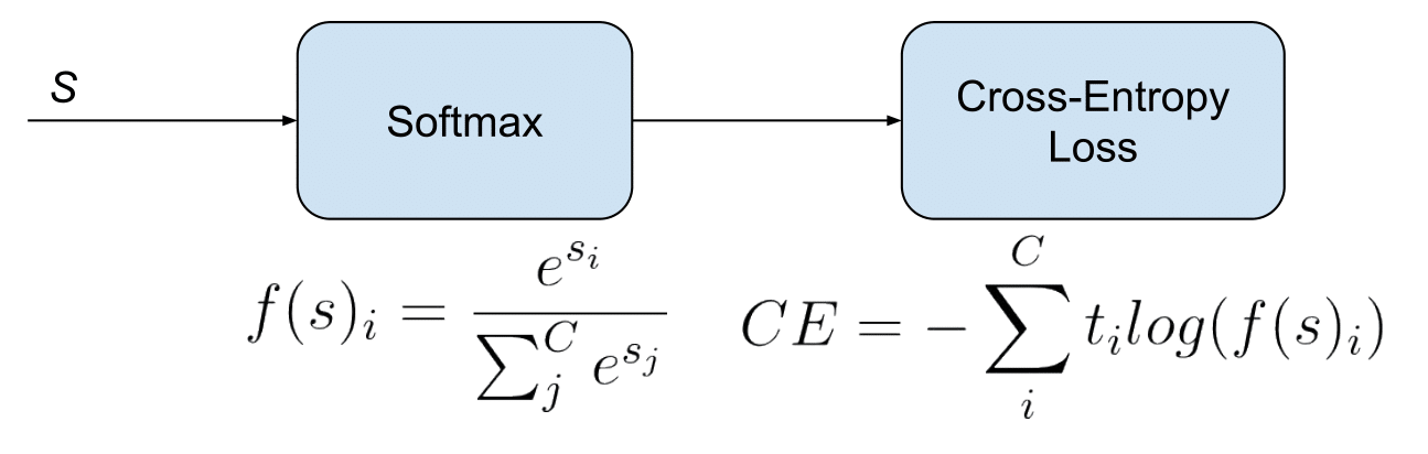
Softmax

Softmax it’s a function, not a loss. It squashes a vector in the range (0, 1) and all the resulting elements add up to 1. It is applied to the output scores $s$. As elements represent a class, they can be interpreted as class probabilities.
The Softmax function cannot be applied independently to each $s_i$, since it depends on all elements of $s$. For a given class $s_i$, the Softmax function can be computed as:

$f(s)_{i} = \frac{e^{s_{i}}}{\sum_{j}^{C} e^{s_{j}}}$

Where $s_j$ are the scores inferred by the net for each class in $C$. Note that the Softmax activation for a class $s_i$ depends on all the scores in $s$.

An extense comparison of this two functions can be found here

Activation functions are used to transform vectors before computing the loss in the training phase. In testing, when the loss is no longer applied, activation functions are also used to get the CNN outputs.

If you prefer video format, I made a video out of this post. Also available in Spanish:

Follow @gombru

Losses

Cross-Entropy loss

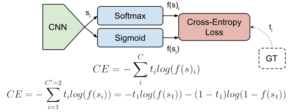
The Cross-Entropy Loss is actually the only loss we are discussing here. The other losses names written in the title are other names or variations of it. The CE Loss is defined as:

$CE = -\sum_{i}^{C}t_{i} log (s_{i})$

Where $t_i$ and $s_i$ are the groundtruth and the CNN score for each class $_i$ in $C$. As usually an activation function (Sigmoid / Softmax) is applied to the scores before the CE Loss computation, we write $f(s_i)$ to refer to the activations.

In a binary classification problem, where $C’ = 2$, the Cross Entropy Loss can be defined also as [discussion]:

$CE = -\sum_{i=1}^{C'=2}t_{i} log (s_{i}) = -t_{1} log(s_{1}) - (1 - t_{1}) log(1 - s_{1})$

Where it’s assumed that there are two classes: $C_1$ and $C_2$. $t_1$ [0,1] and $s_1$ are the groundtruth and the score for $C_1$, and $t_2 = 1 - t_1$ and $s_2 = 1 - s_1$ are the groundtruth and the score for $C_2$. That is the case when we split a Multi-Label classification problem in $C$ binary classification problems. See next Binary Cross-Entropy Loss section for more details.

Logistic Loss and Multinomial Logistic Loss are other names for Cross-Entropy loss. [Discussion]

The layers of Caffe, Pytorch and Tensorflow than use a Cross-Entropy loss without an embedded activation function are:

Caffe: Multinomial Logistic Loss Layer. Is limited to multi-class classification (does not support multiple labels).
Pytorch: BCELoss. Is limited to binary classification (between two classes).
TensorFlow: log_loss.

Categorical Cross-Entropy loss

Also called Softmax Loss. It is a Softmax activation plus a Cross-Entropy loss. If we use this loss, we will train a CNN to output a probability over the $C$ classes for each image. It is used for multi-class classification.

In the specific (and usual) case of Multi-Class classification the labels are one-hot, so only the positive class $C_p$ keeps its term in the loss. There is only one element of the Target vector $t$ which is not zero $t_i = t_p$. So discarding the elements of the summation which are zero due to target labels, we can write:

$CE = -log\left ( \frac{e^{s_{p}}}{\sum_{j}^{C} e^{s_{j}}} \right )$

Where Sp is the CNN score for the positive class.

Defined the loss, now we’ll have to compute its gradient respect to the output neurons of the CNN in order to backpropagate it through the net and optimize the defined loss function tuning the net parameters. So we need to compute the gradient of CE Loss respect each CNN class score in $s$. The loss terms coming from the negative classes are zero. However, the loss gradient respect those negative classes is not cancelled, since the Softmax of the positive class also depends on the negative classes scores.

The gradient expression will be the same for all $C$ except for the ground truth class $C_p$, because the score of $C_p$ ($s_p$) is in the nominator.

After some calculus, the derivative respect to the positive class is:

$\frac{\partial}{\partial s_{p}} \left ( -log\left ( \frac{e^{s_{p}}}{\sum_{j}^{C} e^{s_{j}}} \right ) \right ) = \left ( \frac{e^{s_{p}}}{\sum_{j}^{C}e^{s_{j}}} - 1 \right )$

And the derivative respect to the other (negative) classes is:

$\frac{\partial}{\partial s_{n}} \left (-log\left ( \frac{e^{s_{p}}}{\sum_{j}^{C} e^{s_{j}}} \right ) \right ) = \left ( \frac{e^{s_{n}}}{\sum_{j}^{C}e^{s_{j}}}\right )$

Where $s_n$ is the score of any negative class in $C$ different from $C_p$.

Caffe: SoftmaxWithLoss Layer. Is limited to multi-class classification.
Pytorch: CrossEntropyLoss. Is limited to multi-class classification.
TensorFlow: softmax_cross_entropy. Is limited to multi-class classification.

In this Facebook work they claim that, despite being counter-intuitive, Categorical Cross-Entropy loss, or Softmax loss worked better than Binary Cross-Entropy loss in their multi-label classification problem.

→ Skip this part if you are not interested in Facebook or me using Softmax Loss for multi-label classification, which is not standard.

When Softmax loss is used is a multi-label scenario, the gradients get a bit more complex, since the loss contains an element for each positive class. Consider $M$ are the positive classes of a sample. The CE Loss with Softmax activations would be:

$CE = \frac{1}{M} \sum_{p}^{M} -log\left ( \frac{e^{s_{p}}}{\sum_{j}^{C} e^{s_{j}}} \right )$

Where each $s_p$ in $M$ is the CNN score for each positive class. As in Facebook paper, I introduce a scaling factor $1/M$ to make the loss invariant to the number of positive classes, which may be different per sample.

The gradient has different expressions for positive and negative classes. For positive classes:

$\frac{\partial}{\partial s_{pi}} \left ( \frac{1}{M} \sum_{p}^{M} -log\left ( \frac{e^{s_{p}}}{\sum_{j}^{C} e^{s_{j}}} \right ) \right ) = \frac{1}{M} \left ( \left ( \frac{e^{s_{pi}}}{\sum_{j}^{C}e^{s_{j}}} - 1 \right ) + (M - 1) \frac{e^{s_{pi}}}{\sum_{j}^{C}e^{s_{j}}} \right )$

Where $s_pi$ is the score of any positive class.

For negative classes:

$\frac{\partial}{\partial s_{n}} \left ( \frac{1}{M} \sum_{p}^{M} -log\left ( \frac{e^{s_{p}}}{\sum_{j}^{C} e^{s_{j}}} \right ) \right ) = \frac{e^{s_{n}}}{\sum_{j}^{C}e^{s_{j}}}$

This expressions are easily inferable from the single-label gradient expressions.

As Caffe Softmax with Loss layer nor Multinomial Logistic Loss Layer accept multi-label targets, I implemented my own PyCaffe Softmax loss layer, following the specifications of the Facebook paper. Caffe python layers let’s us easily customize the operations done in the forward and backward passes of the layer:

Forward pass: Loss computation

def forward(self, bottom, top):
   labels = bottom[1].data
   scores = bottom[0].data
   # Normalizing to avoid instability
   scores -= np.max(scores, axis=1, keepdims=True)  
   # Compute Softmax activations
   exp_scores = np.exp(scores)
   probs = exp_scores / np.sum(exp_scores, axis=1, keepdims=True) 
   logprobs = np.zeros([bottom[0].num,1])
   # Compute cross-entropy loss
   for r in range(bottom[0].num): # For each element in the batch
       scale_factor = 1 / float(np.count_nonzero(labels[r, :]))
       for c in range(len(labels[r,:])): # For each class 
           if labels[r,c] != 0:  # Positive classes
               logprobs[r] += -np.log(probs[r,c]) * labels[r,c] * scale_factor # We sum the loss per class for each element of the batch

   data_loss = np.sum(logprobs) / bottom[0].num

   self.diff[...] = probs  # Store softmax activations
   top[0].data[...] = data_loss # Store loss

We first compute Softmax activations for each class and store them in probs. Then we compute the loss for each image in the batch considering there might be more than one positive label. We use an scale_factor ($M$) and we also multiply losses by the labels, which can be binary or real numbers, so they can be used for instance to introduce class balancing. The batch loss will be the mean loss of the elements in the batch. We then save the data_loss to display it and the probs to use them in the backward pass.

Backward pass: Gradients computation

def backward(self, top, propagate_down, bottom):
   delta = self.diff   # If the class label is 0, the gradient is equal to probs
   labels = bottom[1].data
   for r in range(bottom[0].num):  # For each element in the batch
       scale_factor = 1 / float(np.count_nonzero(labels[r, :]))
       for c in range(len(labels[r,:])):  # For each class
           if labels[r, c] != 0:  # If positive class
               delta[r, c] = scale_factor * (delta[r, c] - 1) + (1 - scale_factor) * delta[r, c]
   bottom[0].diff[...] = delta / bottom[0].num

In the backward pass we need to compute the gradients of each element of the batch respect to each one of the classes scores $s$. As the gradient for all the classes $C$ except positive classes $M$ is equal to probs, we assign probs values to delta. For the positive classes in $M$ we subtract 1 to the corresponding probs value and use scale_factor to match the gradient expression. We compute the mean gradients of all the batch to run the backpropagation.

The Caffe Python layer of this Softmax loss supporting a multi-label setup with real numbers labels is available here

Binary Cross-Entropy Loss

Also called Sigmoid Cross-Entropy loss. It is a Sigmoid activation plus a Cross-Entropy loss. Unlike Softmax loss it is independent for each vector component (class), meaning that the loss computed for every CNN output vector component is not affected by other component values. That’s why it is used for multi-label classification, were the insight of an element belonging to a certain class should not influence the decision for another class. It’s called Binary Cross-Entropy Loss because it sets up a binary classification problem between $C’ = 2$ classes for every class in $C$, as explained above. So when using this Loss, the formulation of Cross Entroypy Loss for binary problems is often used:

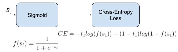
$CE = -\sum_{i=1}^{C'=2}t_{i} log (f(s_{i})) = -t_{1} log(f(s_{1})) - (1 - t_{1}) log(1 - f(s_{1}))$

This would be the pipeline for each one of the $C$ clases. We set $C$ independent binary classification problems $(C’ = 2)$. Then we sum up the loss over the different binary problems: We sum up the gradients of every binary problem to backpropagate, and the losses to monitor the global loss. $s_1$ and $t_1$ are the score and the gorundtruth label for the class $C_1$, which is also the class $C_i$ in $C$. $s_2 = 1 - s_1$ and $t_2 = 1 - t_1$ are the score and the groundtruth label of the class $C_2$, which is not a “class” in our original problem with $C$ classes, but a class we create to set up the binary problem with $C_1 = C_i$. We can understand it as a background class.

The loss can be expressed as:

$CE = \left\{\begin{matrix} & - log(f(s_{1})) & & if & t_{1} = 1 \\ & - log(1 - f(s_{1})) & & if & t_{1} = 0 \end{matrix}\right.$

Where $t_1 = 1$ means that the class $C_1 = C_i$ is positive for this sample.

In this case, the activation function does not depend in scores of other classes in $C$ more than $C_1 = C_i$. So the gradient respect to the each score $s_i$ in $s$ will only depend on the loss given by its binary problem.

The gradient respect to the score $s_i = s_1$ can be written as:

$\frac{\partial}{\partial s_{i}} \left ( CE(f(s_{i})\right) = t_{1} (f(s_{1}) - 1) + (1 - t_{1}) f(s_{1})$

Where $f()$ is the sigmoid function. It can also be written as:

$\frac{\partial}{\partial s_{i}} \left ( CE(f(s_{i})\right) = \begin{Bmatrix} f(s_{i}) - 1 && if & t_{i} = 1\\ f(s_{i}) && if & t_{i} = 0 \end{Bmatrix}$

Refer here for a detailed loss derivation.

Focal Loss

Focal Loss was introduced by Lin et al., from Facebook, in this paper. They claim to improve one-stage object detectors using Focal Loss to train a detector they name RetinaNet. Focal loss is a Cross-Entropy Loss that weighs the contribution of each sample to the loss based in the classification error. The idea is that, if a sample is already classified correctly by the CNN, its contribution to the loss decreases. With this strategy, they claim to solve the problem of class imbalance by making the loss implicitly focus in those problematic classes.
Moreover, they also weight the contribution of each class to the lose in a more explicit class balancing. They use Sigmoid activations, so Focal loss could also be considered a Binary Cross-Entropy Loss. We define it for each binary problem as:

$FL = -\sum_{i=1}^{C=2}(1 - s_{i})^{\gamma }t_{i} log (s_{i})$

Where $(1 - s_i)\gamma$, with the focusing parameter $\gamma >= 0$, is a modulating factor to reduce the influence of correctly classified samples in the loss. With $\gamma = 0$, Focal Loss is equivalent to Binary Cross Entropy Loss.

The loss can be also defined as :

$FL = \left\{\begin{matrix} & - (1 - s_{1})^{\gamma }log(s_{1}) & & if & t_{1} = 1 \\ & - (1 - (1 - s_{1}))^{\gamma } log(1 - s_{1}) & & if & t_{1} = 0 \end{matrix}\right.$

Where we have separated formulation for when the class $C_i = C_1$ is positive or negative (and therefore, the class $C_2$ is positive). As before, we have $s_2 = 1 - s_1$ and $t2 = 1 - t_1$.

The gradient gets a bit more complex due to the inclusion of the modulating factor $(1 - s_i)\gamma$ in the loss formulation, but it can be deduced using the Binary Cross-Entropy gradient expression.

In case $C_i$ is positive ($t_i = 1$), the gradient expression is:

$\frac{\partial}{\partial s_{i}} \left ( FL(f(s_{i})) \right ) = (1 - f(s_{i}))^{\gamma }(\gamma f(s_{i}) log(f(s_{i})) + f(s_{i}) - 1) \quad if \quad t_{1} = 1$

Where $f()$ is the sigmoid function. To get the gradient expression for a negative $C_i (t_i = 0$), we just need to replace $f(s_i)$ with $(1 - f(s_i))$ in the expression above.

Notice that, if the modulating factor $\gamma = 0$, the loss is equivalent to the CE Loss, and we end up with the same gradient expression.

I implemented Focal Loss in a PyCaffe layer:

Forward pass: Loss computation

def forward(self, bottom, top):
   labels = bottom[1].data
   scores = bottom[0].data
   scores =  1 / (1 + np.exp(-scores)) # Compute sigmoid activations
   logprobs = np.zeros([bottom[0].num, 1])

   # Compute cross-entropy loss
   for r in range(bottom[0].num):  # For each element in the batch
       for c in range(len(labels[r, :])):
           # For each class we compute the binary cross-entropy loss
           # We sum the loss per class for each element of the batch
           if labels[r, c] == 0: # Loss form for negative classes
               logprobs[r] += self.class_balances[str(c+1)] * -np.log(1-scores[r, c]) * scores[r, c] ** self.focusing_parameter
           else: # Loss form for positive classes
               logprobs[r] += self.class_balances[str(c+1)] * -np.log(scores[r, c]) * (1 - scores[r, c]) ** self.focusing_parameter
               # The class balancing factor can be included in labels by using scaled real values instead of binary labels.

   data_loss = np.sum(logprobs) / bottom[0].num
   top[0].data[...] = data_loss

Where logprobs[r] stores, per each element of the batch, the sum of the binary cross entropy per each class. The focusing_parameter is $\gamma$, which by default is 2 and should be defined as a layer parameter in the net prototxt. The class_balances can be used to introduce different loss contributions per class, as they do in the Facebook paper.

Backward pass: Gradients computation

def backward(self, top, propagate_down, bottom):
   delta = np.zeros_like(bottom[0].data, dtype=np.float32) 
   labels = bottom[1].data
   scores = bottom[0].data
   # Compute sigmoid activations
   scores =  1 / (1 + np.exp(-scores))

   

   for r in range(bottom[0].num):  # For each element in the batch
       for c in range(len(labels[r, :])):  # For each class
           p = scores[r, c]
           if labels[r, c] == 0:
               delta[r, c] = self.class_balances[str(c+1)] * -(p ** self.focusing_parameter) * ((self.focusing_parameter - p * self.focusing_parameter) * np.log(1-p) - p) # Gradient for classes with negative labels
           else:  # If the class label != 0
               delta[r, c] = self.class_balances[str(c+1)] * (((1 - p) ** self.focusing_parameter) * (
               self.focusing_parameter * p * np.log(
                   p) + p - 1))  # Gradient for classes with positive labels

   bottom[0].diff[...] = delta / bottom[0].num

The Focal Loss Caffe python layer is available here.

Additional Resources

Keras Loss Functions Guide: Keras Loss Functions: Everything You Need To Know

Follow @gombru