About my Participation in the WebVision Challenge
The WebVision Challenge was a competition organized in conjunction with the CVPR2017. It’s an ImageNet like competition, where the participants have to classify the images between the 1000 ImageNet classes. The Top-5 accuracy is the ranking metric. The difference is that the systems have to learn only from web data. To do that the WebVision dataset is presented.
The dataset
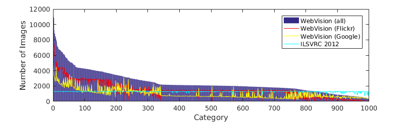
The WebVision dataset It’s a dataset formed by 2.4M images compiled from Google images and Flickr. The images were obtained by making queries with the imagenet class names to these platforms. So the query text is the label of each image, and those labels are quite noisy. In addition to the label, the images are accompanied with other metadata. Regarding text, Google images are accompanied by the image (“alt”) description and the page title, and Flickr images are also accompanied by hashtags. The original images are available, but in this experiments I used the resized dataset, where images smaller side is always 256px.
Using the textual information to learn from noisy-labeled data
I participated in this competition to test how textual information accompanying images in the web can be used to learn. In this case we have predefined classes and a noisy label for each image, so the idea is to use the text to supervise those labels in the learning pipeline.
I tried 2 different strategies:
- Train a CNN weighting the label of each sample depending on how much its associated text is related with the class.
- Train a CNN with 2 heads, one classification head that takes into account the labels and one regression head that takes into account the text.
But first I filtered the dataset removing the noisy samples and trained a CNN with the clean dataset. I used that model as a pretraining for the other two strategies.
All the code used (python and Caffe) is available here.
Technical setup
Hardware
Since I was working with web data, I knew about the competition when it was released. But I was busy with other work and didn’t have powerful enough hardware to participate. But just 3 weeks before the submissions deadline in the lab we received a cluster with 4 Nvidia GeForce® GTX 1080 Ti (Intel Core i7-5820K CPU @ 3.30GHz, 64GB RAM, 2x500GB SSD, 8TB HD) we had bought some weeks ago. So to learn how to use the cluster fast and test it I decided to participate in the competition.
Software
I’m still more fluent with Caffe than with TensorFlow so I decided to use it. Also I wanted to build some complex nets that would be tedious to code in TensorFlow. Ovemore, Caffe just released their Multi-GPU support for pyCaffe and people were saying it worked like a charm (see this GitHub merge).
About the CNN, I decided to use GoogleNet. I recently had tried to fine-tune a ResNet, but I had trouble for that (and many people were having with ResNets in Caffe). There are many models working better than GoogleNet out there, but the difference is small, and since I was handling that net, knew its training behaviour and only had 3 weeks, I decided to use it. Anyway my plan was not to win the competition, it was just to learn how to use the cluster and to explore different ways to use the text associated to images in the learning process.
Training a deep CNN from scratch
People usually fine-tune models pre-trained on ImageNet instead of training them from scratch. That’s useful because with that pretraining the net learns to extract general features useful for any model. Then adapting the net to classify other classes or solve other problems is faster and easier. Sometimes only the last layers need to be re-trained.
But in this challenge the objective is to test the performance of a model that has learnt solely from web data (free data). So using pre-trained models is not allowed. Training a “small” model as AlexNet from scratch can be done in 1 day, but training a GoogleNet is another story. So I decided to train a single model from scratch using a cleaned dataset (see the section “Cleaning the dataset”). Then, I will fine-tune this model to test the proposed strategies.
To do the pretraining I used LMDB. Using this database to read the images has some benefits. It’s the fastest way to read from disk. It stores images in raw format so they can be read directly and don’t have to be processed after that. They are read directly and don’t have to be loaded to RAM. The drawback is that they are huge, like 10-20 times jpg data.
The code I used to create the LMDB is available here.
The training set (after discarding noisy images) weighted 36GB (jpg images with the shorter side of 256px). The LMDB weighted 500GB (images resized to 256x256, since building a LMDB os images of different sizes is tricky).
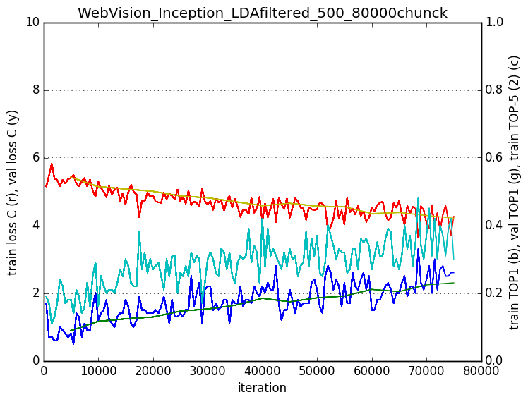
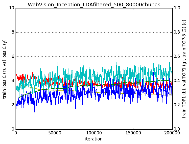
So I put the training LMDB in the empty SSD (filled it), the validation LMDB in the system SSD and started training. I used a batch size of 80 (the bigger one that fitted in a GPU) in each of the 4 GPU’s, so that’s an effective batch size of 320. I used SGD and tried to set a higher learning rate than 0.01 (the default one when training GoogleNet with batch size of 32), but the gradient exploded. The momentum was 0.9 and the weight decay 0.0002. As data augmentation I used random cropping of 227x227 patches and mirroring (both are provided by Caffe for LMDB). The time per iteration was 200ms. Reading data from LMDB is a SSD is free.
The rule that Facebook stated (If you increase the batch size by k, you can increase the learning rate by k and you’ll get the same performance) was not fulfilled here. I couldn’t increase the learning rate despite using a bigger batch size. Though, the learning was less noisy using a big batch size.
Cleaning the dataset
I trained an LDA with the text associated to training images. You can read an explanation about the LDA and the details about its training in this post (the explained procedure is the same one used here). The LDA basically creates topics from the training text taking into account which words appear together in the text pieces. Those topics have a semantic sense. For instance, one topic can gather words about cooking and another one about sports. Then the LDA can infer a topic distribution for any piece of text. That topic distributions codes how a piece of text is related to each one of the topics. So the idea is to discard those images whose associated text topic distribution is not related to the class. The number of topics used was 500.
With the trained LDA, we computed the topic distribution of the texts associated to training images. Then we computed the mean topic distribution of each class. Finally, we computed the cosine similarity between the mean topic distribution of each class and each of the samples of that class, and score the samples with it. So we had a value associated to each training image, measuring how much is related the image associated text to the class. To remove the noisy samples of the dataset, we set a threshold and discard those samples with a similarity value below it.
For instance we might want images of “Queen” but get a photo of the Queen rock band. The mean topic distribution of the class would have high values for topics related to royalty and history stuff, but the topic distribution of the text associated with the Queen rock band will be very different, having high values for topics related to music. So we would discard that image.
It’s a very simple method, but the noise removal was effective, especially for some classes that have a name that can generate confusions between two objects, or for classes that have a lot of noise because there are few images results of them in google or flickr. We discarded the 10% of the training set. For the classes containing few samples, we were less restrictive.
Some examples of the discarded images for some classes:
For the class 0: “Tench”
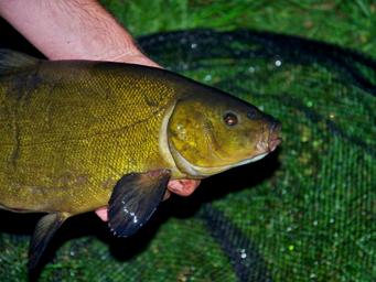
We discarded:
For the class 300: “tiger beetle”
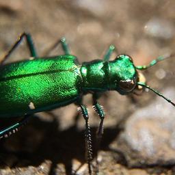
We discarded:
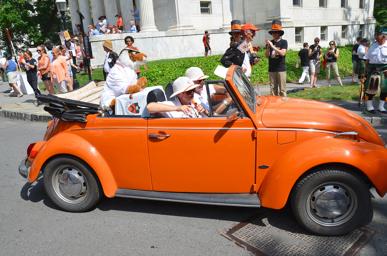
For the class 800: “slot, one-armed bandit”

We discarded:

Strategy 1: Using soft-labels
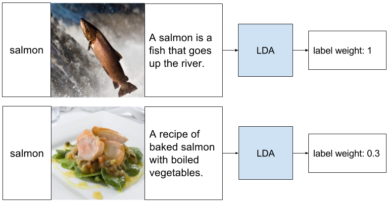
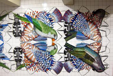
As we have explained, the text associated to an image can give a clue about if the label assigned to it is correct or not. That information can be used taking profit of the LDA. This strategy, instead of discarding those images whose associated text has a topic distribution which is not similar to the mean of the class, generates a confidence for each label based on that. Let’s explain it with the example in the figure: We have previously trained an LDA with all the training text and computed the mean topic distribution of the text associated to the images of the class “salmon”. Then, for each image associated to this class, we compute the topic distribution of its associated text, and compute the cosine similarity with the mean of the class “salmon”. If the image contains a salmon fish (which is the kind of images we want for the class), the text will probably talk about fishes, rivers… so it will have a topic distribution similar to the mean of the class, and we can trust its label “salmon” and assign to it a weight of 1. But if the text associated to the image talks about cooking, its topic distribution will be very different from the mean of the class, so we cannot trust the label that much, we will assign it a weight λ of 0.3.
We call this weighted labels soft labels. The idea is giving in the training procedure more importance to those labels with a high confidence λ. So the net uses a higher learning rate when we are sure that the image contains a salmon fish, but a lower one when we are not sure because it may contain a salmon dish, a T-shirt of salmon color, or whatever.
Softmax loss with soft labels
To learn using soft labels we create a custom softmax loss were the contribution of each sample to the loss is weighted.
Given the softmax loss:
Where \(C\) are the classes to be inferred [0-999], \(i\) is the GT class, \(s_j\) are the scores inferred by the net for each class and \(s_i\) is the score inferred by the net for the GT class. We want to add a scalar λ that weights the loss for each sample depending in how reliable its label is. So we want a softmax loss with soft labels:
Defined the loss, now we have to minimize it. We’ll do so with gradient descent. To do that we evaluate the gradient of the loss function with respect to the parameters, so that we know how we should change the parameters to decrease the loss. So we need to compute the gradient respect each \(s_j\), which are the scores given by the net for each clas. The gradient expression will be the same for all \(C\) except for the GT class \(i\), because the score of the GT class \(s_i\) is in the nominator.
After some calculus, the derivative respect to the GT score \(s_i\) is:
And the derivative respect to the other classes would be:
Where \(k\) is a class from \(C\) different from \(i\).
Softmax loss with soft labels: Coding it in Caffe
Now let’s see how to translate this equations to code in Caffe (PyCaffe). We use a python layer that let’s us easily customize the operations done in the forward and backward passes of the layer.
Forward pass: Loss computation
def forward(self, bottom, top):
   labels_scores = bottom[2].data
   labels = bottom[1].data
   scores = bottom[0].data
   #normalizing to avoid instability
   scores -= np.max(scores, axis=1, keepdims=True)
   exp_scores = np.exp(scores)
   probs = exp_scores / np.sum(exp_scores, axis=1, keepdims=True)

   correct_logprobs = np.zeros([bottom[0].num,1])
   for r in range(bottom[0].num):
       correct_logprobs[r] = -np.log(probs[r,int(labels[r])]) * labels_scores[r]

   data_loss = np.sum(correct_logprobs) / bottom[0].num

   self.diff[...] = probs
   top[0].data[...] = data_loss
For each image of the batch, we have one label score λ, one label \(i\), and a score for each one of the classes \(C\) \(s_j\). So we compute the softmax loss for each image of the batch and multiply it by the label score. The batch loss will be the mean loss of the elements in the batch. We then save the data_loss to display it and the probs to use them in the backward pass.
Backward pass: Gradients computation
def backward(self, top, propagate_down, bottom):
   delta = self.diff
   labels = bottom[1].data
   labels_scores = bottom[2].data
   for r in range(bottom[0].num):
         delta[r, int(labels[r])] -= 1
         delta[r,:] *= labels_scores[r]
   bottom[i].diff[...] = delta / bottom[0].num
In the backward pass we need to compute the gradients of each element of the batch respect to each one of the classes scores \(s_j\). As the gradient for all the classes \(C\) except the GT class \(i\) is equal to probs λ, we assign probs values to delta. Then for the Gt class \(i\) (int(labels[r])) we subtract 1 to match the gradient expression. Finally we multiply all the gradient expressions by the labels scores λ. We compute the mean gradients of all the batch to run the backpropagation.
The Caffe Python layer of this softmax loss using soft labels is available here.
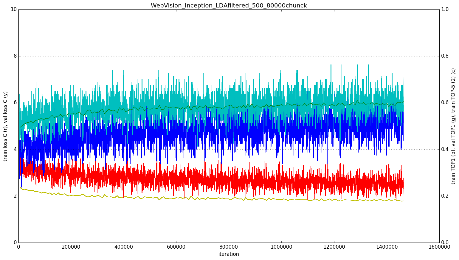
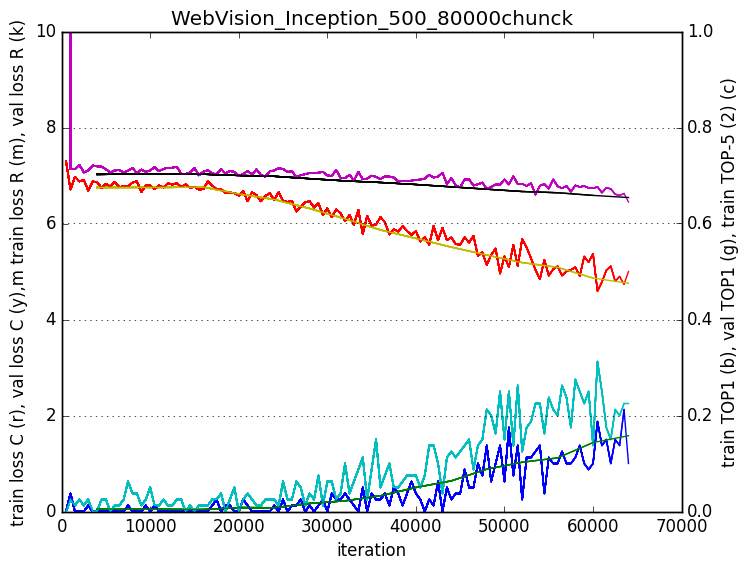
I continued training the model using the softmax loss with soft labels from the LMDB trained one. The model continued learning as slow as it was learning in the late LMDB training, so I cannot say with certainty if this strategy helped or not.
Strategy 2: 2-headed CNN
This strategy uses a CNN with two different losses:
- The classification head learns to classify the images to its GT class.
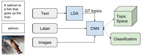
- The regression head learns to assign to each image the LDA topic distribution given by its associated text.
We give a larger weight to the classification head (the used values were [0.75,0.25]) because it’s the objective task. The idea is that the regression head supervises the classification head. Let’s see how it works with an example:
We are training our net and we receive an image of a salmon fish labeled as “salmon”. The LDA topic distribution of its associated text will probably be similar to other salmon fish images. The loss of the classification head will shift the weights to predict the salmon class when that image is received (GOOD!). The loss of the regression head will shift the weights to predict the topic distribution given by the associated text, which will be similar to the one given by other salmon fish images (GOOD!). So the net would learn weights that when a salmon image is given infer the salmon label and the salmon associated topic distribution. Now let’s imagine that the net receives an image of a salmon-colored T-shirt. The LDA topic distribution of its associated text will probably be very different to salmon dish images. The classification loss will shift the weights to predict the salmon class when that image is received (BAD! -that’s a T-shirt, not a fish-). The loss of the regression head will shift the weights to predict the topic distribution given by the associated text, which will be similar to the one given by other T-shirt images (GOOD!).
It’s hard to think about this and to reason if it could work. But when the idea is that the net receives an image of a salmon-colored T-shirt with the label “salmon” (which is noise) the classification Loss would be changing the weights wrongly to predict the salmon class from a T-shirt image, but the regression Loss would be changing the weights in the correct direction despite the incorrect label.
Net design
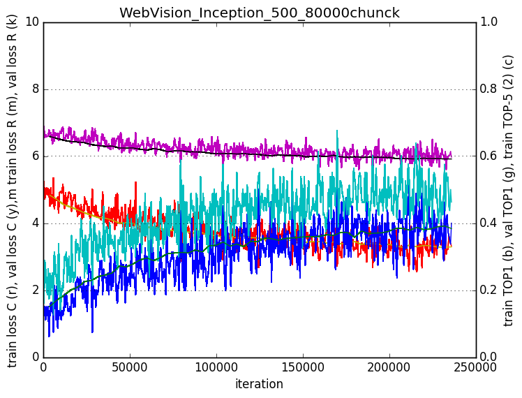
I built this 2 headed CNN over GoogleNet. I added a regression head next to each one of the 3 classification heads, so actually the net has 6 losses. I duplicated the fully connected layers preceding the heads, learning separate weights for the regression and the classification. I used sigmoid cross entropy loss to learn the regression. I weighted the weights giving 0.75 to the classification head and 0.25 to the regression head (and respecting the weights that GoogleNet uses for the heads at the different net stages). Later I thought that probably I should use a lower weight in the regression head, but couldn’t try it.
Results
The classification results were much better for the strategy 1 than for the strategy 2. However, using an ensemble of these two classifiers helped. I also found out that evaluating different patches of the same image provided a boost in the results. The boost provided by this techniques in the Imagenet challenge are explained by google in the Inception paper.
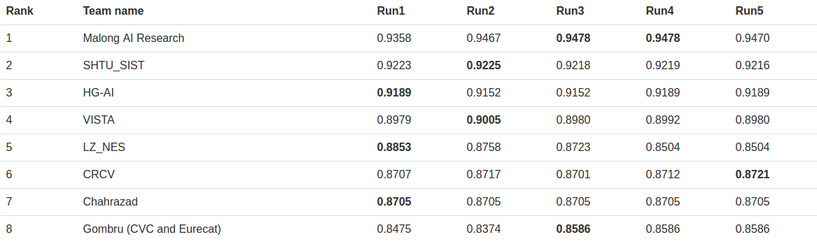
The table shows the results of the competition. I was the last one. Having a look to the descriptions of the other participant methods, I have to say that I didn’t balance the data, and that was my mistake. Other differences is that they all used more recent CNN models. Also, some of them used different CNN models trained on the noisy dataset and then used their predictions to filter the noise and train the final model instead of using the text associated to images.
Conclusions
The experience of participating in this competition has been interesting and enriching. My two objectives were, first, explore how the textual information can be used to learn better from noisy labeled data, second, learn how to use the multi-GPU cluster. I focused in those two objectives, and probably that was why I didn’t get better results.
Probably taking care of more basic strategies as data balancing and focusing on using the current top performing ImageNet model would have lead to better results, as the pipeline and the results of other participants show. Also considering from the beginning more competition-oriented techniques, as classifier ensembling, instead of exploring how could I increase the learning rate by using a bigger batch size splited in the 4 GPUS. However, I do not regret of the work done, since the objective was learning and not winning the competition.
Another conclusion that could be extracted from here is that when we have labels, even though they are noisy, the CNN training can deal with it. However we will have to see the full explanations of the winning methods to state that.